Block Diagram Reduction Rules – Control System

We have discussed in our previous article that for the easiness of analysis of a control system, we use block diagram representation of the control system. Basically we know that a complex system is difficult to analyze as various factors are associated with it.

Thus it is always better to draw the block diagram of the system in the easiest possible way thereby making the analysis simple.

But as we also know that the block diagram representation of a system involves summing points, functional blocks, and take-off points connected through branches and flow of signal shown by the arrowheads.

In the previous section, we have seen a simple form of a closed-loop system that has single forward and feedback blocks with the inclusion of a summing and a take-off point.

However, when we deal with control systems, then we come across various complex block diagram representation of systems that holds various functional blocks with multiple summing points and take-off points.

So, such a complex diagram must be reduced to its simple or canonical form. However, while reducing the block diagram it is to be kept in mind that the output of the system must not be altered and the feedback should not be disturbed. So, to reduce the block diagram, proper logic must be used.

Hence for the reduction of a complicated block diagram into a simple one, a certain set of rules must be applied. Here in this section, we will discuss the rules needed to be followed.

Rules for Block Diagram Reduction

So, one by one we will discuss the various rules that can be applied for simplifying a complex block diagram.

For serially connected blocks

When blocks are connected in series then the overall transfer function of all the blocks is the multiplication of the transfer function of each separate block in the connection.

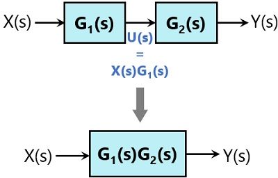
Suppose we have two blocks in cascade connection as shown below:

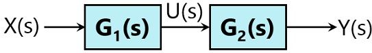
Consider U(s) denotes the intermediate variable then we can say

and

Hence

Thus we can replace two blocks with different transfer functions into a single one having the transfer function equal to multiplication of each transfer function without altering the output.

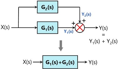
For parallely connected blocks

In case the blocks are connected parallely then the transfer function of the whole system will be the addition of the transfer function of each block (considering sign).

Suppose two blocks are connected parallely as given below:

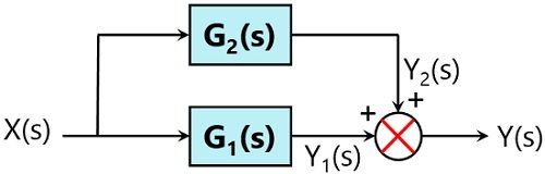
So,

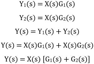
So, two parallely connected blocks can be replaced by a single block with a summation of the transfer function of each block.

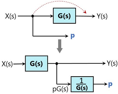
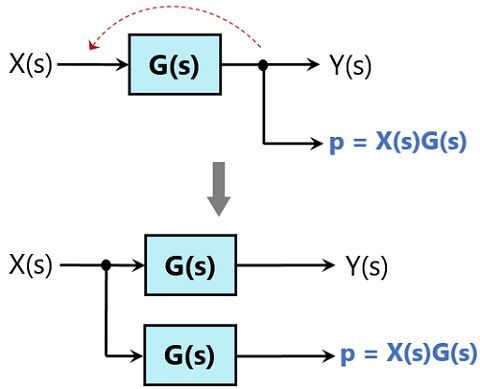
Shifting of take-off point ahead of the block

Suppose we have a combination of take-off point and block as shown below:

If we need to shift the take-off point ahead of the block, then we must keep ‘p’ as it is.

Here p = X(s)

So, even after shifting p must be X(s) and for this, we have to add a block with gain which is reciprocal of the gain of the originally present block.

As the actual gain is G(s) so the additional block will have a gain of 1/G(s).

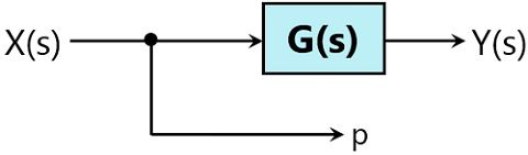
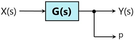
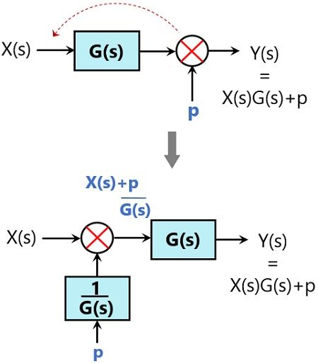
Shifting of take-off point behind the block

Suppose there is a take-off point ahead of block as given below:

In order to move the take-off point behind the block, we need to keep the value of ‘p’ same. Here p = X(s)G(s).

But with backward movement p will become X(s). So, we have to add another block with the same gain as the original gain. This will make the value of p = X(s)G(s)

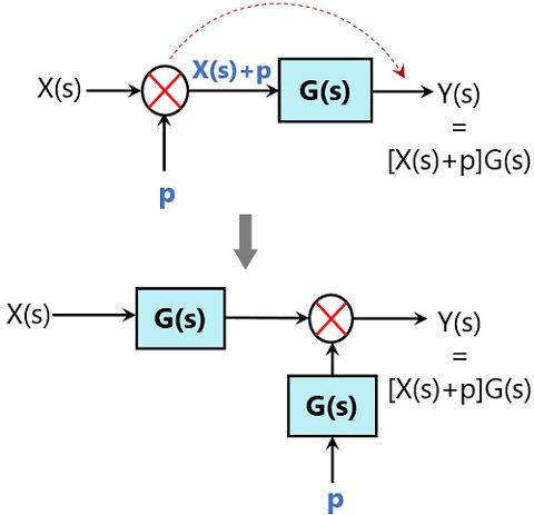
Shifting of Summing point ahead of the block

Suppose we have a configuration of summing point and block as given below:

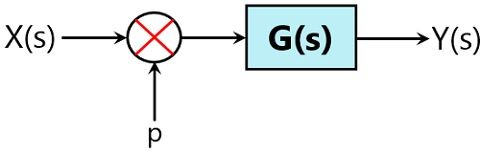
If the summing point is to be moved from backward to forward of the block, then Y(s) will become X(s)G(s)+p. However, earlier Y(s) was [X(s)+p]G(s).

So, to have unaltered output, we need to add a block having exact gain as the original one.

Shifting of summing point behind the block

Suppose we have a combination where we have a summing point present after the block as shown below:

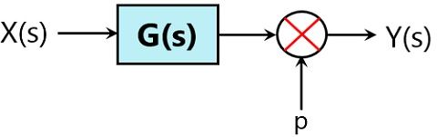
We need to move this summing point behind the position of the block without changing the response. So, for this, a block with gain which is reciprocal of the actual gain is to be inserted in the configuration in series.

Interchange of the summing point

Consider a combination of two summing points directly connected with each other as shown below:

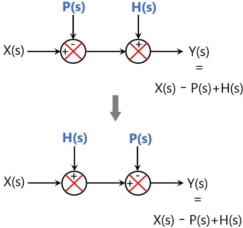
We can use associative property and can interchange these directly connected summing points without altering the output.

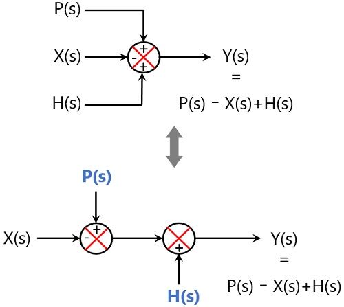
Splitting/ combining the summing point

A summing point having 3 inputs can be split into a configuration having 2 summing points with separated inputs without disturbing the output. Or three summing points can be combined to form a single summing point with the consideration of each given input.

The figure below shows the above-discussed configuration:

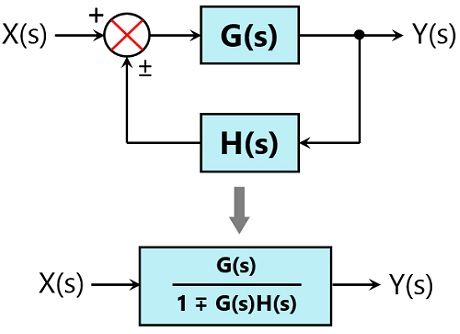
Eliminating the feedback loop

We have already derived in our previous article that the gain of a closed-loop system with positive feedback is defined as:

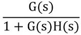
So to remove the feedback loop, feedback gain must be used.

Therefore, we can have:

Example of Block Diagram Reduction

Till now we have seen the important rules to be kept in mind while reducing the block diagram. Let us now see an example to have a better understanding of the same.

First, see the procedural steps to be followed for solving block diagram reduction problems:

1. The directly connected blocks in series must be reduced to a single block.
2. Further, reduce the parallely connected block into a single block.
3. Now reduce the internally connected minor feedback loops.
4. If shifting does not increase the complexity, then try having the take-off point towards the right while summing point towards left.
5. Repeat the above-discussed steps to have a simplified system.
6. Now determine the transfer function of the overall closed-loop simplified system.

Consider a closed-loop system shown here and find the transfer function of the system: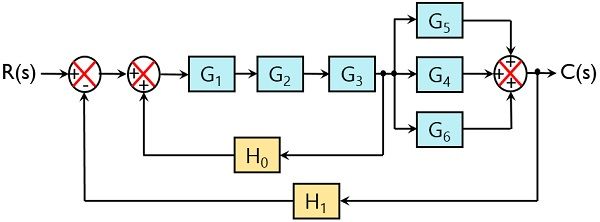

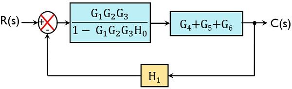
Reducing the 3 directly connected blocks in series into a single block, we will have:

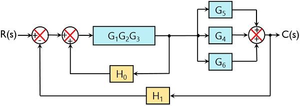
Further, we can see 3 blocks are present that are connected parallely. Thus on reducing blocks in parallel, we will have:

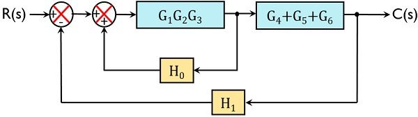
Further on simplifying the internal closed-loop system, the overall internal gain will be

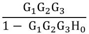
So, we will have:

Now reducing the two blocks in series:

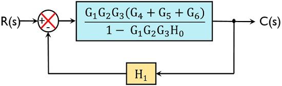
So, this is the reduced canonical form of a closed-loop system.

We know gain of the closed-loop system is given as:

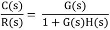
Therefore,

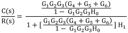
On simplifying the equation

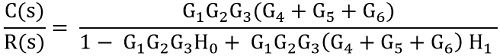
This is the overall transfer function of the given control system.