Root Locus is a way of determining the stability of a control system. In the previous article, we have discussed the root locus technique that tells about the rules that are followed for constructing the root locus.
Here in this article, we will see some examples regarding the construction of root locus. But before going these solved examples you must have the basic idea about the rules for constructing the root locus. So, first, go through the article root locus technique.
Before proceeding towards the examples let us see what steps are needed to be followed to draw root locus from the transfer function of the system.
General Steps to Draw Root Locus
1. Firstly, from the given transfer function of the system, the characteristic equation must be written through which the number of open loop poles and zeros must be determined. On getting the number of poles and zeros, depending on the rule, the total number of branches is determined.
2. Now, the poles-zero plot must be drawn. Once the s-plane plot is formed then the sections of real axis where the root locus exists is determined. Also, through general predictions, the minimum number of breakaway points is predicted simultaneously.
3. Next, the calculation of the angle of asymptotes for the various branches is done using the formula.
4. The point of intersection of asymptotes on the real axis of s-plane is known as the centroid which is to be calculated further by the desired formula. Now a draw a sketch till the centroid to get the rough idea about the construction of locus.
5. Further, the breakaway point is to be determined using the method for its determination. And in case, it appears to be complex conjugates then its validity must be checked using angle condition.
6. Determine the points intersecting of root locus with the imaginary axis.
7. If applicable with the conditions derived from the above rules then calculate the angle of arrival and departure.
8. With the above-specified steps and obtained values, construct a final sketch of root locus. Now, by observing the root locus, predict the stability and performance of the system.
Examples for Construction of Root Locus
Here in this section, we will see some examples that will help you to understand how the root locus is drawn for a system to check its stability.
Example1: Suppose we have given the transfer function of the closed system as:![]()
We have to construct the root locus for this system and predict the stability of the same.
Firstly, writing the characteristic equation of the above system,![]()
So, from the above equation, we get, s = 0, -5 and -10.
Thus, P = 3, Z = 0 and since P > Z therefore, the number of branches will be equal to the number of poles.
So, N = P = 3
Thus, under this condition, the branches will start from the locations of 0, -5 and -10 in the s-plane and will approach infinity.
Initially, with general prediction, we can say that the point -5 on the real axis has an odd sum of total number of poles and zeros to the right of it. Thus, in between 0 and -5 there will be one breakaway point.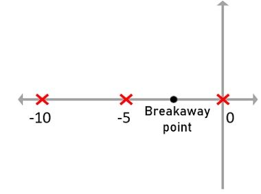
Now, let us calculate the angle of asymptotes with the formula given below: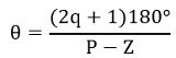
: q lies between 0 to P-Z-1
So, in this case, θ will be calculated for q = 0, 1 and 2.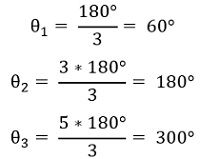
So, these three are the angle possessed by asymptotes approaching infinity.
Now, let us check where the centroid lies on the real axis by using the formula given below:
The figure below represents a rough sketch of the plot that is obtained by the above analysis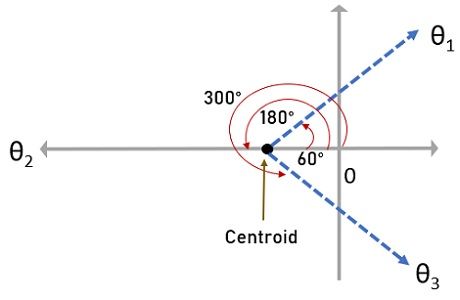
Earlier we have predicted that one breakaway point will be present in the section between points 0 and -5. So, now using the method to determine the breakaway point we will check the validity of the breakaway point.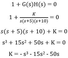
In this method, roots obtained on differentiating K with respect to s and equating it to 0, will be the breakaway point.
Therefore,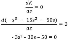
Or![]()
Thus, on solving, roots obtained will be -2.113 and -7.88.
As the root -7.88 falls beyond the predicted section for the breakaway point thus s = -2.113 is the valid breakaway point.
Further, we can get the value of K on substituting the value of s= -2.113 in the equation,![]()
Therefore, on solving,![]()
Here, K obtained is a positive value, hence, s = -2.113 is valid.
Now, we have to check the at what point the root locus intersects with the imaginary axis. Thus, for this routh array is used.
Here a proper method is used where the characteristic equation is used and routh array in terms of K is formed.![]()
Thus, the Routh’s Array: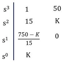
Now, to find Kmar, which is the value of K from one of the rows of routh’s array as row of zeros, except the row s0.
Considering, row s1, 750 – K = 0
Thus, Km = 750
Further, with the help of coefficients of the row which is present above the row of zero, an auxiliary equation A(s) = 0 is constructed. In this case,![]()
So, substituting the value of Km in the above equation, we will get,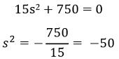
Therefore,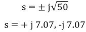
Thus, these are the intersection points of the root locus with the imaginary axis.
Also, as the poles are not complex thus angles of departure not needed. Hence, at the breakaway point, the root locus breaks at ± 90°.
So, the complete root locus is given below: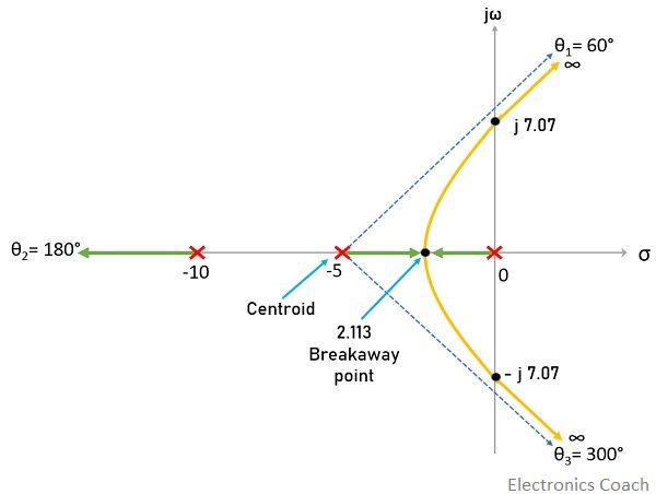
From the above sketch, the stability of the system can be analyzed that for K between 0 to 750 the system is completely stable as the complete root locus lies in the left half of s-plane. While at K = 750, the system is marginally stable.
While, for K between 750 to ∞, the system is unstable as the dominant roots proceed towards the right half of s-plane.
Example2: Consider that for the system with transfer function given below we have to sketch the root locus and predict its stability.![]()
The characteristic equation provides the poles and zeros. So, writing the characteristic equation for the above system:![]()
Thus, s = 0,![]()
On solving
s = – 1 + j and -1 – j
Thus, here
P = 3, Z = 0 and as P > Z, so rule wise N = P = 3
The pole-zero plot is given below: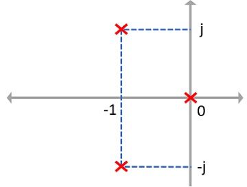
Here, it is clear that branch originating from s = 0 approaches -∞. And general predictions clear that there is no breakaway point here.
Angle of asymptotes
Since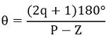
: q lies between 0 to P-Z-1
So, here, θ will be calculated for q = 0, 1 and 2.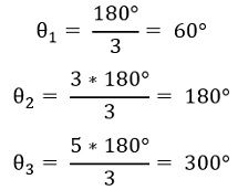
Now, centroid: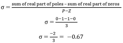
So, with the help of the above analysis, the sketch of s-plane is given below: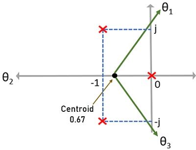
With angle θ2, one branch from s = 0 approaches to infinity and with θ1 and θ3, branches starting from -1+j and -1-j respectively, approach infinity.
Now, let us check for the breakaway point.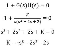
So, on differentiating,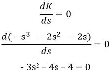
Or![]()
Breakaway points are calculated as:![]()
Therefore,
s = – 0.67 ± j 0.47
Now, as here we are having complex conjugates, thus, checking the validity of these points as breakaway point by using angle condition.
Testing, s = – 0.67 + j 0.47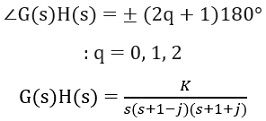
At s = – 0.67 + j 0.47![]()
On solving,![]()
As it is not an odd multiple of 180° thus, this point is not present on the root locus, hence there is no breakaway point here.
Further, checking for the intersection with the imaginary axis.![]()
Routh’s array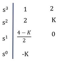
The value of Km = +4 makes s1 = 0
Thus,![]()
Substituting Km = 4, we get,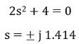
Now, calculating angle of departure
At complex pole, – 1 + j![]()
So, here φP1 = 135° and φP2 = 90°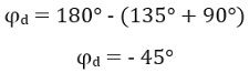
Therefore, at the complex pole, – 1 – j,![]()
So, with the above-determined values and parameters, the complete root locus sketch obtained is given below: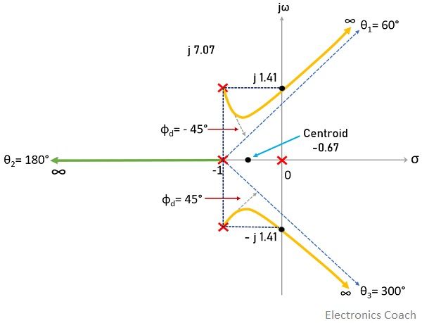
Now talking about stability, for K between 0 to 4, the roots are present on the left half of s-plane, representing a completely stable system.
K = +4 makes the system marginally stable due to the presence of dominant roots on the imaginary axis. While for K > 4, the system becomes unstable as dominant roots lie in the right half of s-plane.
Thus, in this way by plotting the root locus, the stability of the system can be determined.
Leave a Reply