Root Locus Technique

In the previous article, we have discussed the basics of root locus. Basically, the root locus technique or plot is a way of constructing root locus that involves some rules as it helps in determining the stability of the control system.

We have discussed that the graph formed by plotting the path of the roots of the characteristic equation obtained for various values of K is root locus. This simply helps in determining the values of K that satisfies the complete performance of the system thereby providing a stabilized system for operation.

Rules for Constructing Root Locus

For higher-order systems, the root locus must be constructed with certain rules keeping in mind. The rules for constructing the root locus are as follows:

1. Symmetricity of root locus

The roots of the characteristic equation of the system can be either real, complex or combination of both.

So, suppose we have n number of roots for K between 0 to infinity, the root locus on the s-plane must exhibit symmetricity about the real axis of the s-plane.

2. The starting and termination of root locus

This rule states, the root locus must begin from open-loop poles and must specifically terminate on either open-loop zero or infinity.

Now, under this specific rule, we have to consider two conditions, depending upon the number of open-loop poles i.e., P and number of open-loop zeros i.e., Z.

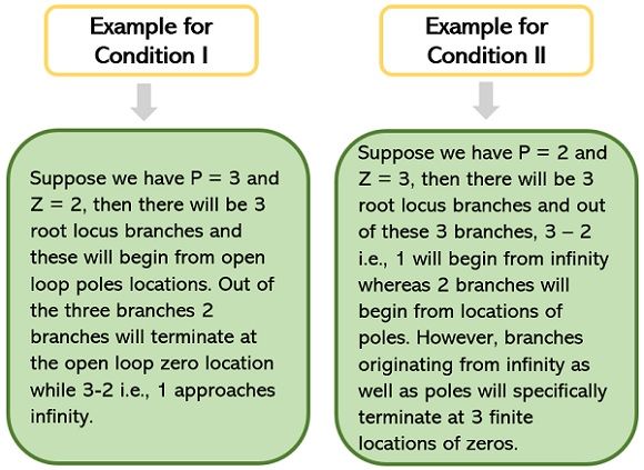
Condition I: If the number of open-loop poles is greater than the number of open-loop zeros i.e., P > Z.

Then the number of branches, N will be equivalent to the number of poles, P. So, for P branches originating from each pole, Z number of branches will get terminated at the open-loop zero and P-Z number of branches will terminate at infinity.

Condition II: If the number of open-loop poles is smaller than the number of open-loop zeros i.e., Z > P.

Then, the number of branches, N will be the same as the number of zeros, Z. So, for Z branches, P number of branches will get started from open-loop pole locations and Z – P number of branches will start from infinity and approaches the finite zeros.

It is to be noted here that in both the conditions the direction of branches will be from poles towards the zeros.

3. Angle of Asymptotes

In the previous rule we have discussed two conditions of root locus where P > Z or Z > P, but generally, the systems have a greater number of poles than zeros. So, P-Z branches approach infinity. And this rule is related to how these branches approach infinity.

Basically, the branches that approach infinity do so in a fashion of straight line which is called asymptotes of root locus. These are symmetrical about the real axis.

So, the angles at which the asymptotes of the root locus are formed are given as:

: r lies between 0, 1, 2 —– (P – Z – 1)

4. Location of asymptotes in the s-plane

For asymptotes, it is said that there is a common point at which all the asymptotes undergo intersection on the real axis. This point is referred as centroid and is represented by σ.

So, the coordinates where the centroid is present on the real axis is determined by:

It is to be noted for centroid that it may or may not be located on the root locus but is always present on either the negative or positive real axis as it is always of real nature.

5. Root Locus on the real axis

This rule is about the presence of a point on the root locus. Basically, a point on the real axis of the s-plane will be present on the root locus if the overall summation value of open-loop poles and zeros will be odd to the right of this point.

Suppose we have a pole-zero plot given below and we have to check on which part of the real axis, the root locus exists.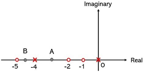

So, consider point A is on the real axis and we have to count the overall poles and zeros to the right of it.

Thus, as there are 1 pole and 2 zeros to the right of this point hence the sum is odd thus A is on the root locus. Also, as point A lies between s = -2 and s = -4, so for any location of point A within this section, the real axis will be a part of root locus.

Furthermore, if we consider point B, then to the right of this point, the overall poles and zeros are 4 i.e., even. Thus, rule wise this point is not a part of root locus. However, if this point shifts to a location beyond -5 on the above-given plot then the condition will get change as the inclusion of s = -5 will make the sum odd again.

Due to this reason, this rule is applied to different sections of the pole-zero plot in order to check the existence of the various sections of the s-plane on the root locus.

6. Breakaway Point

Breakaway point is always present on the root locus and indicates a point where various roots of the characteristic equation occur keeping K at a specific value.

To understand this, consider the plot shown below: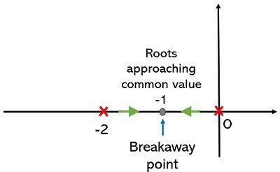

Here the section between pole 0 and -2 is present on the root locus thus according to rule at least one breakaway point is present here.

This is so because the two different values of s begin from the respective open-loop pole locations and approach a common value i.e., s = -1 when K rises from 0 to 1. This point at K=1, here is a breakaway point. Further from this particular point, the roots breakaway as a pair of complex conjugates when K approaches infinity.

Also, the breakaway is always present on the root locus and from the above plot, it is clear that to the right side of that point, only one pole is present signifying odd value for the sum of poles and zeros which is discussed in rule 5.

7. Angle of departure 

We know branch originates from an open-loop pole thus the angle at which it departs from the complex conjugate pole is known as angle of departure. Denoted as φ_d.

The angle of departure of root locus from a complex pole is given as: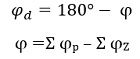

where

 Σ φ_p is the sum of angles formed by vectors drawn from other poles at the pole where the angle of departure is to be calculated,

Σ φ_Z is the summation of the angles made by vectors drawn from zeros at the pole.

8. Intersection of root locus with the imaginary axis of the s-plane

If the root locus crosses the imaginary axis then the point of intersection on the root locus can be determined by applying Routh-Hurwitz criteria. To find the point for the value of K where the root locus crosses the imaginary axis, the terms in the first column of the Routh array are equated to zero.

In the upcoming article, we will see how these rules are implemented while constructing the root locus with the help of examples.