Definition: The transfer function of a control system is the ratio of Laplace transform of output to that of the input while taking the initial conditions, as 0. Basically it provides a relationship between input and output of the system.
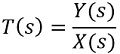
For a control system, T(s) generally represents the transfer function.
In the figure given below X(s) and Y(s) represents input and output respectively.
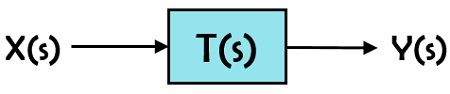
The transfer of the system is given as:
Transfer function is considered as an appropriate way of representing a linear time-invariant system.
We know that in a control system, the way in which the system behaves on applying input causes the variation in output.
For any system, initially, the parameters of the system are defined and according to the need of the system, the values are selected. Further, the input is selected to determine how the system is performing.
So, the output achieved will represent the performance of the system. Thus can be expressed as:
Thus
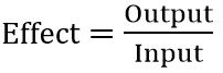
Thus we can say that it is a mathematical function explaining the system parameters according to the applied input so as to get the desired output.
The open-loop and the closed-loop system have a different transfer function. This is so because the feedback loop gets introduced in a closed-loop system.
Terms related to the Transfer Function of a System
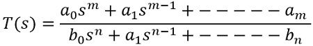
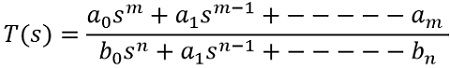
As we know that transfer function is given as the Laplace transform of output and input. And so is represented as the ratio of polynomials in ‘s’.
Thus, can be written as:
In the factorized form the above equation can be written as:
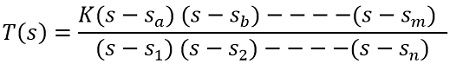
: k is the gain factor of the system.
- Poles of Transfer Function
Poles of the transfer function are defined as those values of the parameter ‘s’ whose substitution in the denominator makes the transfer function as infinite.
So, in the above equation, if s is substituted as s1, s2 — sn in the denominator, then these values act as the poles of the transfer function.
When the term in the denominator is equated to zero then the obtained roots are known as poles.
Let we have a system with transfer function:
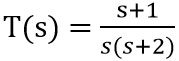
To have poles of the transfer function
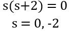
These are the poles of the above transfer function. As the substitution of these values in the denominator leads to provide infinite transfer function.
The poles of a transfer function generally are of three types: simple, repeated and conjugate poles.
If the values are real and non-repetitive, then such poles are known as simple poles.
Example: s = 0, 2, -4 etc.
While when the values of the poles are repetitive then such poles are known as repeated poles.
Example: s = -1, +1, -2, -2 etc.
Whereas when there exist complex conjugate values of the poles then it is known as complex conjugate poles.
Example: s = -2 + j1
The x-axis in the s-plane represents the poles.
- Zeros of Transfer Function
We have already discussed that poles are specified by the denominator of the transfer function. However, the zeros of the transfer function are evaluated using the numerator.
Those values of the s that when substituted in the numerator of the transfer function make the transfer function zero, is known as zeros of that transfer function.
Like the poles, the zeros are also roots of the equation, which is achieved when the term in the numerator is equated to 0.
The zeros can also be of 3 types depending upon, whether they are repetitive, non-repetitive or complex conjugate pairs.
Consider that a system has a transfer function:
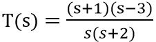
To have zeros of the transfer function
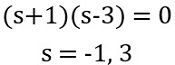
These are the zeros of the transfer function, as these values on substitution make the overall transfer function of the system 0.
- Characteristic Equation of Transfer Function
The denominator of the transfer function of the system, when equated to 0, provides the characteristic equation of that particular system.
For transfer function:
The characteristic equation will be given as:
![]()
- Order of Transfer Function
The order of the transfer function is defined by the characteristic equation of the system. It is basically the maximum power of s which is present in the characteristic equation (i.e., in the denominator polynomial).
- Pole-Zero Plot
When all the poles and zeros of the transfer function are represented in the s-plane. Then such a plot is known as a pole-zero plot of the system.
- DC gain
Whenever the frequency component of the transfer function i.e., ‘s’ is substituted as 0 in the transfer function of the system, then the achieved value is known as dc gain.
Procedure to calculate the transfer function of the Control System
In order to determine the transfer function of any network or system, the steps are as follows:
- Firstly, the time domain equations of the system must be written after considering different required variables in the system.
- Then after considering the initial conditions as zero, write the Laplace transform of the time domain equations of the system.
- Now determine the input as well as output variables from the frequency domain equations i.e., the Laplace transform.
- Further, the initially considered variables must be removed and we have to write the resultant equations in the form of input and output variables.
- Now, the ratio of Laplace transform of output and input must be determined in order to have the transfer function of the overall system.
As we have already discussed that Laplace transform acts as the major step in determining the transfer function of an electrical network. We know that most electrical network consists of elements like R, L, and C.
The table is given below shows the time domain and frequency domain expression for voltage of elements R, L and C.
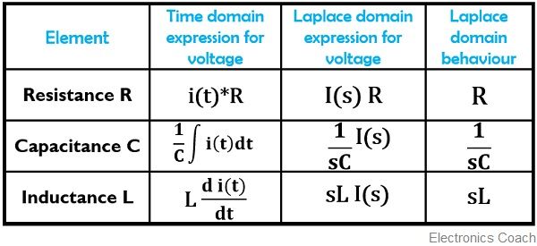
So, by the use of Laplace domain expression, the transfer function of any electrical network consisting of R, L and C can be determined.
Consider the electrical network given below whose transfer function is to be determined:
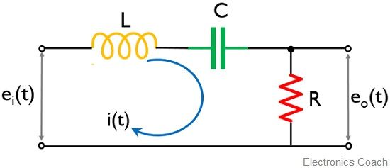
Let ei(t) and eo(t) be the input applied and output of the circuit respectively.
On applying KVL in the above circuit,
![]()
and
![]()
Further neglecting the initial conditions and taking Laplace transform of the above equations, we will get
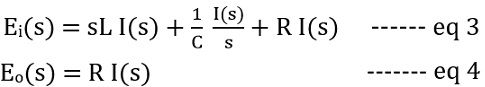
Thus
![]()
As I(s) is an introduced variable so we need to convert it in the form of input and output.
From eq4
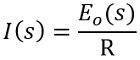
Substituting the value of I(s) in eq 5, we will get
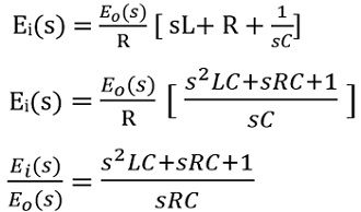
As transfer function is the ratio of output by input in the Laplace domain.
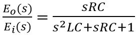
Thus, this is the transfer function of the above given electrical network.
Advantages
- The complex time-domain equations can be converted into simple algebraic form using Laplace transform.
- It provides the mathematical model of the overall system along with each system component.
- For a known transfer function, the output response is easy to determine for any reference input.
- It helps to determine important parameters of the system like poles, zeros, etc.
- The stability of the system can be easily analyzed using the transfer function.
- It helps to relate output with input.
Disadvantages
- It is not applicable to non-linear systems.
- The initial conditions are not considered as the effects generated by them are neglected.
This is all about the transfer function of a control system.
Leave a Reply