The analysis of a control system is done in a way to determine the variation in output with respect to the input. Basically the response of any control system can be analyzed in frequency as well as time domain.
So, the analysis of a system that involves defining input, output and other variables of the system as a function of time is known as time-domain analysis.
It is also known as the time response of the control system. This is so because the response is defined as the output provided by the system when certain excitation is given to it. Thus time response of the control system provides the idea about the variation in the output of the system with respect to time.
Control systems are considered a dynamic system and time is considered as an independent variable in most of the systems. Thus analyzing the response of the system as a function of time is quite necessary.
Time Response of Control System
Time response of the system is defined as the response of the system achieved on providing certain excitation, where the excitation and response must be a function of time.
We know that a physical system is composed of energy-storing components like an inductor, capacitor, etc. The presence of such elements in the system causes some delay whenever there is any requirement for changing the energy state of the system.
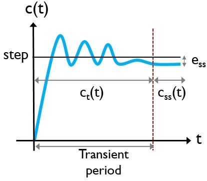
Due to this reason when certain excitation is provided to the system then it takes some time to achieve the desired output. However, before achieving the desired value, the output of the system fluctuates to the nearby value. This leads to a classification of the time response of the control system.
So, the time response of a control system is classified as:
- Transient response: It is defined as the response of the system as the variation in output of the system before achieving the final value when excited with the input signal.
We know that when an input is applied to the system, then it takes some time in order to attain the final value. But before attaining the final value, the output of the system varies nearly around a finite range.
This change in the output of the system, to a finite range on applying input, is known as a Transient response.
Thus we can say that the output of the system, before the actual value, is known as a transient response. As the transient response is not the final value thus the time taken by the system to attain the desired value is known as a transient period.
This means the variation in output which is nothing but the transient response, decays to 0 with time.
The transient response is generally expressed as ct(t) and can be of either exponential or oscillatory nature.
- Steady-state response: The actual value of the time response, that is achieved after the elimination of the transient response is known as a steady-state response.
Hence we can say that the final value of output provided by the system, according to the applied excitation is known as a steady-state response.
This means after the exhaustion of the transient response, the specifically achieved output for the input is referred as a steady-state response.
It is denoted as Css.
So, the overall time response can be given as:
![]()
Thus
It is not always necessary that achieved output is absolutely the desired one. As sometimes there exists some variation from the desired output.
The steady-state error provides the information regarding the variation of the achieved output from that of the desired output. This is so because it is the difference between the desired value and achieved value.
Thus this response gives an idea about the accuracy of the system.
Standard Test Inputs
Basically there exists a wide range of time-varying signals like ramp, square, sawtooth, triangular, rectangular, etc. Thus these signals can act as the reference input for the control system. So, as we have a large range of time-varying signals thus considering each one of them for the purpose of the analysis is quite difficult.
Therefore, we use some time-varying signals that act as reference input and these signals are known as standard test inputs.
Thus a system is basically evaluated by the response provided by it to the standard inputs.
Step Input: A signal which is applied at a particular time is known as step input.
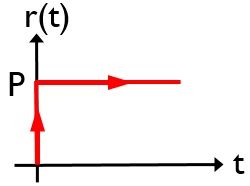
The step input is mathematically expressed as:
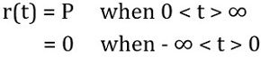
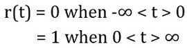
For the unit step function, the value of P will be equal to 1.
Thus unit step function is mathematically expressed as:
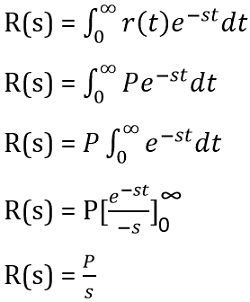
The Laplace transform of the step function will be:
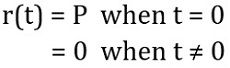
Impulse Input: A signal of very high amplitude which is applied for only a short period of time represents an impulse function. When the amplitude of the signal is 1, then it is said to be unit impulse function.
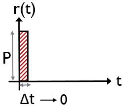
It is mathematically expressed as:
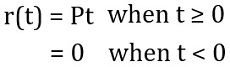
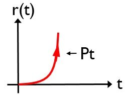
Ramp Input: A signal that shows a constant variation in the input with time represents a ramp function. More simply, it is a constant rate of change of input, thus shows a gradual increase.
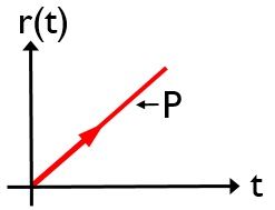
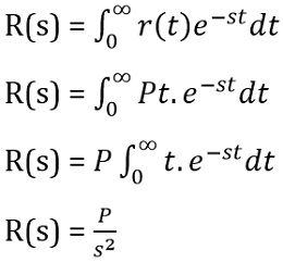
The ramp signal is mathematically expressed as:
The Laplace transform of the ramp function:
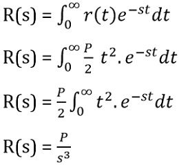
Parabolic Input: Parabolic functions are referred as the functions which are somewhat a degree faster in comparison to ramp type.
The mathematical representation of a parabolic function is given as:
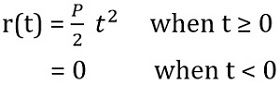
: P represents the magnitude of parabolic input.
The Laplace transform of the parabolic function will be:
Hence we can say that the time-domain analysis of a control system represents the response of the system with variation in time.
Leave a Reply