Time Response of Second Order System

The type of system whose denominator of the transfer function holds 2 as the highest power of ‘s’ is known as second-order system. This simply means the maximal power of ‘s’ in the characteristic equation (denominator of transfer function) specifies the order of the control system.

The order of the system provides the idea about closed-loop poles of the system.

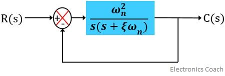
The block diagram of the second-order system with unity feedback is given below:

Introduction

We have already discussed in time domain analysis of control system that every practical system needs a finite amount of time before attaining the actual output. As before reaching the final values, the system undergoes oscillations due to which the output fluctuates.

This is the reason the overall time response of the control system is the combination of steady-state response and transient response. And is given as:

The steady-state response is the final value of the output while the transient response is the response due to oscillations.

It is noteworthy here that during the transient period, the system undergoes exponential increase or starts oscillations. But the type of closed-loop poles and their position in the s-plane are responsible for the way in which system behaves.

When a certain input is applied and the system starts to oscillate then in order to get the final output that oscillatory behaviour must be opposed.

So, the effect that tends to obstruct or resist the oscillatory behaviour of the system so as to attain the final value is known as Damping.

Damping controls the type of closed-loop poles and is measured using the damping ratio. The damping ratio is expressed as ξ.

Thus we can say that the damping ratio defines how dominant the system is towards the generated oscillations and this ratio varies from system to system.

In some system, the damping ratio is quite low, thus such systems oscillate slowly. While some system exhibits a high damping ratio, where the output despite oscillating rises exponentially. Thus in such systems, the system slowly reaches the steady-state.

If the damping ratio is 0, then there will be an absence of restriction by the system to the oscillations. Thus, in this case, the system oscillates with maximum frequency. And the frequency of oscillations at ξ = 0, is the natural frequency of oscillations. It is denoted by ω_n.

Time Response of Second Order System

The open-loop gain of the second-order system is given as:

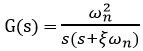
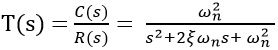
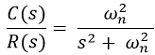
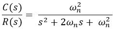
We know that the transfer function of a closed-loop control system is given as:

So, the closed-loop gain of the control system with unity negative feedback will be:

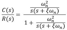
On simplifying, we get,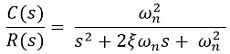

This is the transfer function of a standard 2^nd order system. Thus the characteristic equation will be:

Practically for a system, the value of numerator can be a constant or polynomial other than ω_n². However, in the denominator, the middle and the last term coefficients must be as it is.

Thus to have the values of ω_n and ξ, the denominator of the transfer function must be compared with the standard form.

Let us first find the roots. So, consider the characteristic equation:

Further

On substituting, we will get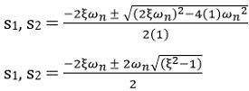

On simplifying

If ξ = 0

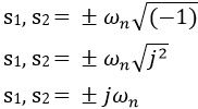
So, for ξ = 0, the roots are purely imaginary.

Further if ξ = 1

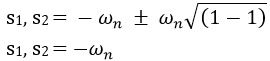
For, ξ = 1, the roots are purely real. And such a system is critically damped.

Furthermore in the case of

0 < ξ < 1

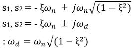
For ξ > 1

In this condition, the system is said to be overdamped.

Time Response of Second-Order system with Unit Step Input

Let us first understand the time response of the undamped second-order system:

We know the basic transfer function is given as:

As we have already discussed that in the case of the undamped system

ξ = 0

So, the transfer function of the undamped system will be given as:

We know that for unit step signal,

r(t) = u(t) for t ≥ 0

Therefore,

Since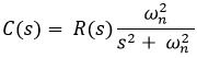

On substituting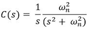

Taking partial fraction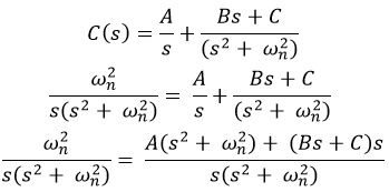

On simplifying

Comparing the constant

Comparing the coefficient of s²

Comparing the coefficient of s

Substituting the values in the partial fraction, we will get

Taking Inverse Laplace transform of the over equation

Thus

This is the time response of the undamped second-order system with a unit step input.

The figure below represents the response of the undamped system: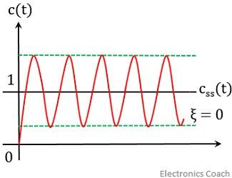

Let us now consider critically damped second order system:

In case of a critically damped system,

ξ = 1

So, the transfer function of the critically damped system:

In the case of unit step signal,

r(t) = u(t) for t ≥ 0

Thus,

As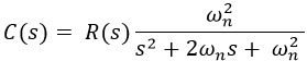

On substituting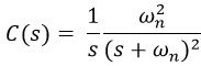

Taking partial fraction

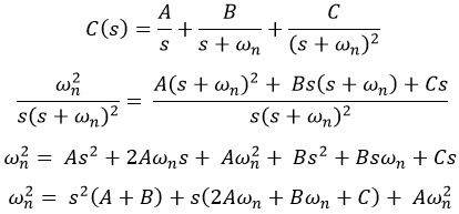
Comparing the constant

Comparing the coefficients of s²

Further comparing the coefficient of s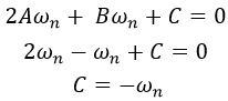

Now on substituting the values in partial fraction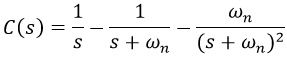

Taking inverse Laplace transform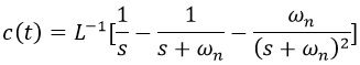

Thus, we will get

This is the time response of the critically damped second-order system with a unit step input.