It is a technique used for finding the transfer function of a control system. Basically, a formula that determines the transfer function of a linear system by making use of the signal flow graph is known as Mason’s Gain Formula.
It shows its significance in determining the relationship between input and output.
Introduction
In the previous article, we have seen how a signal flow graph is constructed. We have already seen that a signal flow is a graph is generally formed by using the algebraic equations that define the system, in which the variables of the equations play a crucial role.
Previously we have discussed that S J Mason introduced the idea of signal flow graph to make the analysis of the system easy. Also, the formula for finding the transfer function of the SFG was stated by Mason. Thus, it is named so.
In the block diagram reduction technique, we have seen that in order to simplify a system for the purpose of analysis, we must apply some reduction rules in a proper manner. And after the simplification of the system, its overall transfer function C(s)/R(s) is determined.
This means that to simplify the system, after applying each rule, a reduced block diagram must be formed after every step. This makes the simplification time-consuming.
So, to deal with the problems regarding block diagram reduction, signal flow graph is adopted and used.
In SFG, once the graph is obtained then the transfer function can be easily determined by mason’s gain formula.
Mason’s Gain Formula
To determine the transfer function of the system using signal flow graph, the formula given below is used.![]()
Here every term has its own significance, as these values vary with signal flow graph.
K denotes the number of forward paths,
TK shows the gain of the kth forward path,
Δ is the determinant of the system calculated as:
Δ = 1 – (sum of loop gains of total individual loops in the SFG) + (sum of the product of gains of all pairs of two non-touching loop in SFG) + (sum of the product of all pairs of three non-touching loops in the SFG) + ——
ΔK denotes the Δ for the region of SFG which do not touches the Kth forward path.
We will see the application of mason’s gain formula on the signal flow graph using some examples but first, let us understand the different terms associated with the mason’s gain formula.
So, basically by noticing the above formula, we get the idea that firstly the total number of forward paths in the graph must be calculated as this will play a crucial role in determining the overall gain between input and output of the system.
Further, all the number of loops in the SFG must be noted down with their respective gain as their summation is required. Also, the gains of each loop in the SFG must be summed but only those with two non-touching loops.
In a similar way, the combination of gains with three non-touching loops must be summed. This continues till the SFG contains even higher number of non-touching loops.
Once this all is determined, then by substituting the respective gains in the above-described formula, the overall gain of the signal flow graph is determined and so the system.
Let us now see some examples.
Examples of Mason’s Gain Formula
In the previous article, we have already described the way to construct a signal flow graph.
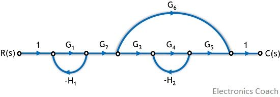
So, now consider that we have a signal flow graph shown below and we have to determine its respective gain.
- Example 1:
Here we will apply mason’s gain formula but first, determine each component of the formula step by step.
Here the total number of forward paths are two.
T1 = G1G2G3G4G5
T2 = G1G2G6
Also, the above signal flow graph contains, 2 individual feedback loops
L1 = – G1H1
L2 = – G4H2
These two loops of the SFG are also the two non-touching loops.
Therefore, substituting the values in the formula to calculate Δ, we will get,
Δ = 1 – (L1 + L2) + (L1L2)
Δ = 1 – (- G1H1 – G4H2) + [(- G1H1) (- G4H2)]
So,
Δ = 1 + G1H1 + G4H2 + [(G1G4 H1H2)]
Further, we will now calculate ΔK
So,
Δ1 = 1 – (loops that are not touching first forward path)
And here there is no such loop which is not touching the first forward path, hence,
Δ1 = 1 – (0)
Δ1 = 1
Now,
Δ2 = 1 – (loops not touching the second forward path)
And here L2 is not touching the second forward path, therefore,
Δ2 = 1 – (L2)
Δ2 = 1 – (- G4H2)
On simplifying
Δ2 = 1 + G4H2
So, now substituting the values in the mason’s gain formula: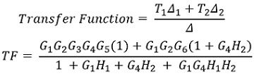
This is the gain of the system with the above given SFG.
- Example 2:
Consider the SFG shown below: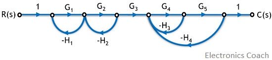
Here we have only a single forward path.
Thus, K = 1
So,
T1 = G1G2G3G4G5
The 4 individual feedback loops of the above shown signal flow graph are:
L1 = – G1H1
L2 = – G2H2
L3 = – G4H3
L4 = – G4G5H4
The various combinations of 2 non-touching loop of the SFG are:
L1L3 = (- G1H1)(- G4H3) = G1H1G4H3
L1L4 = (-G1H1)(-G4G5H4) = G1H1G4G5H4
L2L3= (-G2H2)(-G4H3) = G2H2G4H3
L2L4= (-G2H2)(-G4G5H4) = G2H2G4G5H4
In this SFG, there are no 3 non-touching loops, thus we will stop right here.
So, Δ will be given as:
Δ = 1 – (-G1H1 – G2H2 – G4H3– G4G5H4) + [(G1H1G4H3) + (G1H1G4G5H4) + (G2H2G4H3) + (G2H2G4G5H4)]
So, we will have,
Δ = 1 + G1H1 + G2H2 + G4H3 + G4G5H4 + G1H1G4H3 + G1H1G4G5H4 + G2H2G4H3 + G2H2G4G5H4
Now, as we have a single forward path,
Therefore, Δ1 = 1 – (0)
This is so because we have no such loops that are not touching the first forward path.
So, Δ1 = 1
Hence, the transfer function of the above signal flow graph will be:![]()
On substituting the values, we will get,
![]()
This is the transfer function of the system with the above-given signal flow graph.
Hence, in this way, the input relationship of a complex system using signal flow graph can be determined.
Yellaiah Bachali says
very clean explanation and easy understanding